Determining the radiant of a meteor using Graves radar

Important
This article has been superseded by this one: http://ea4eoz.blogspot.com/2016/04/determining-radiant-of-meteor-using.html

During the last months of 2014, Iban EB3FRN and me were recording meteor head echoes using Graves. But to make things interesting, we synchronized the recordings using a PPS GPS signal. The idea was to analyze the Doppler from the head echoes and and see if something useful can be extracted from them.

Typical Graves' head echo followed by a large tail echo

On paper, the procedure was easy: We recorded a stereo wav file, with the output from the receiver in one channel, and a PPS signal in the other channel. Then, both wav were synced using those PPS signals into a simple stereo wav, with one receiver in each channel.

Reality was quite different. Do you think your sound card record sound at the specified sample rate? No, it doesn't. They are sightly off, and the sample rate drifts with time. We are talking of errors about 0.2 to 0.5 samples per second, enough to be noticed after some hours.

After resampling the wav files to 48000.000 samples per second, and align them, we finally get more than 60 hours of double station Graves recordings made during the nights of August 30 to 31, November 16 to 17 and 17 to 18 (Leonids) and December 13 to 14 (Geminids).

A lot of interesting things can be heard in those 60 hours, but this time we were looking for head echoes received at both locations at the same time. We found 62 head echoes received simultaneously on both locations, and you can see / watch them in this video (better with headphones).

The video was made with Baudline, rotating the image to get the better look of time on horizontal axis, and frequency on vertical axis. The green signal is the audio received at Iban's station (EB3FRN) and the red one is the signal received by me (EA4EOZ)

As expected, the Doppler signature is different at each location, and we know how that Doppler signature is produced. The Doppler value, this is the instantaneous Doppler value of head echo reflection is a function of meteor position and velocity vector, and the relative vector positions to the transmitter and receiver sites:

and the Doppler slope, this is the rate of change of the Doppler value is:

where:

     Vm is the meteor velocity vector, in km/s
     Mtx is the position vector from the meteor to the transmitting site, in km.
     Mrx is the position vector from the meteor to the receiving site, in km.
     F is the transmitting frequency, in Hz. 143050000 Hz for Graves.
     c is the speed of light, in km/s.
     And · denotes the dot product between vectors.

The problem is these two formulas have no inverse. You can calculate the Doppler and the Doppler slope from a known meteor at a given position with a given velocity, but you can't calculate meteor position and velocity from the Doppler values. One of the reasons is these formulas have the dot product. You can calculate the dot product of a pair of vectors, but given a dot product, you can find an infinite number of vectors whose dot product is exactly the same. What does it means? For a given Doppler and Doppler slope you can find an infinite number of meteors that will produce the measured Doppler and Doppler slope.

But what about the Doppler and Doppler slope from two locations? Could it solve the meteor? Or at least, reduce the solution set to something useful? It was worth trying.

I wrote a small Octave script to search for meteor solutions using the above formulas, for example:

The meteor detected on 2014 December 14 03:07:34

 UTC. Note how weak is the red trace.

This meteor were recorded almost at the Geminids' peak, so it is probably a Geminid. At a given time it produced a Doppler of 694 Hz with a slope of -2960 Hz/s at Iban's receiver, and a Doppler of 386 Hz with a slope of -2643 Hz at my location.

The script is an infinite loop that uses Octave's fsolve function to solve the above meteor functions. The solving function tries to solve the above functions from a random starting point (X, Y, Z) with a random velocity vector (Vx, Vy, Vz). Then fsolve varies these input values trying to match the desired result. If fsolve finds a solution, it returns a point in the space Mx, My, Mz, with a velocity vector MVx, MVy, MVz that matches the observed values of Doppler and slope. The script is keept running until it produce a large amount of solutions, usually over 100000 solutions

For convenience, the script also produces some other output data along with the cartesian coordinates, like longitude, latitude and height above sea level ( Mx, My, Mz --> Lon, Lat, Asl ), Velocity ( sqrt (MVx*MVx+MVy*MVy+MVz*MVz) ), Right ascension and declination (Ra, Dec) elevation over local horizon (El), distances from Mx, My, Mz to transmitter and receiver sites (Dtx, Drx1, Drx2), and signal traveled distance (STD1, STD2).

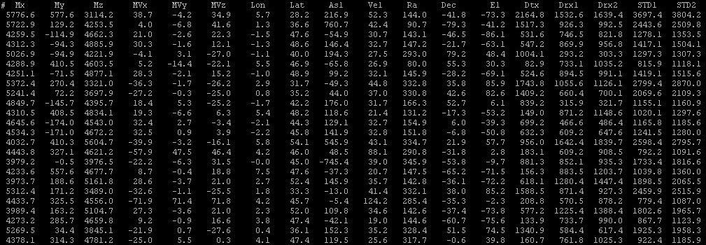
Typical output data for a meteor

If you plot these solutions in 3D, you will find something like this:

Solution set for meteor 20141214-030734

Each red pixel in the above image is a solution of the previous meteor. This is, a meteor placed in that point (Mx, My, Mz), with a given velocity and direction (MVx, MVy, MVz) produces exactly the observed Doppler and Doppler slope at each location.

The figure seems to have some "structure" but interestingly all solutions (possible meteors) are contained in a well delimited area in the space. Analyzing all these solutions in detail it is clear many of them can be discarded, for example:

Position: It can be seen in the image. Some solutions are under ground, and some of them are very high. It is known most meteors burn around 90-100km. Over 100-110 km they are still unburned, so no radio reflection is possible. Under 80km most of them have been disintegrated, so keep solutions between 90 and 100 km seems reasonable.

Velocity: Meteors with velocities under 12 km/s can't keep orbiting the sun, and over 72 km/s will get lost into interstellar space. For a meteor in orbit around the sun, velocity must be between 12 and 72 km/s, so we can discard solutions with velocities under 12 km/s and over 72 km/s

Velocity vector: The meteor must fall from the sky. So we can discard meteors (solutions) "going up", this is, coming from a point under the local horizon.

Distance: Because of earth's size and curvature, a meteor burning in the upper atmosphere can be seen at a given maximum distance. Ham radio operators have determined experimentally that the maximum possible distance using meteor scatter is about 1400 miles, or 2250 km. This means one observer in earth surface can't see a meteor farther than half that value, this is 1125 km. Let's round that number to 1200 km, to allow observers higher than sea level and some possible tropospheric diffraction in the extreme cases. In this way, a possible solution for a meteor, must be under 1200 km for both observers, but it must be also under 1200km from the TX site, in this case, the Graves radar transmitting site. So, we can discard solutions at more than 1200 km to any of the observers, or transmitting site.

Once these "impossible" solutions are discarded, the remaining ones can be plotted into a map:

Meaningful solutions for meteor 20141214-030734

They are aligned along a curve. Each point in this curve is a solution (meteor) having it's own velocity vector (direction and magnitude). Because we know when the meteor was detected (December 14, 2014 03:07:34 UTC) it is easy to plot those velocity vector directions upward into the sky:

Possible radiants of meteor 20141214-030734

The solutions also draw a curve in the sky, and surprisingly, this curve pass over the radiant of the Geminids (AR: 7h 28m, Dec: +33). Looking for the solutions at that point in the sky, all of them are located at longitude 8.1º east, latitude 45.1º north (near Turín, in Italy) with a velocity around 38 km/s. It is interesting to note Geminids have a velocity of 35 km/s.

So, it seems the above meteor was indeed a Geminid, who fall in Italy, near Turin, at 38 km/s.

From all 62 double meteor head echoes detected, only 39 were measurable using Baudline's debugmeasure function:

Meteor	FRN Doppler Hz	FRN Slope Hz/s	EOZ Doppler Hz	EOZ Slope Hz/s
20140830-232422	109	-1453	442	-1397
20140830-235705	51	-1600	185	-2312
20140831-000342	275	-338	317	-314
20140831-012732	514	-1442	196	-990
20140831-032936	-573	-1429	98	-12858
20140831-053212	1404	-8167	290	-7767
20140831-055719	499	-10481	454	-9250
20140831-064706	1698	-6501	1211	-3601
20141117-011331	132	-1978	186	-1623
20141117-023603	1582	-1474	233	-1349
20141117-024613	1100	-3756	300	-3089
20141117-024708	63	-844	386	-720
20141117-030648	151	-845	96	-656
20141117-035358	42	-375	185	-313
20141117-040409	-628	-756	131	-812
20141117-080229	1206	-7223	-51	-1912
20141117-104226	865	-1268	298	-1050
20141117-111112	-309	-2861	144	-2747
20141118-002853	423	-2877	365	-2667
20141118-003124	577	-2368	477	-2368
20141118-023329	875	-4075	343	-3642
20141118-023336	1372	-3788	455	-3434
20141118-031006	309	-6067	378	-5267
20141118-063249	385	-12167	491	-12100
20141118-064155	1545	-8401	809	-11534
20141118-105654	175	-2417	312	-1784
20141214-025158	1168	-1953	487	-1727
20141214-030536	342	-677	179	-1486
20141214-030734	694	-2960	386	-2643
20141214-031451	760	-2645	362	-3401
20141214-031729	1388	-3431	884	-3178
20141214-032346	775	-2783	207	-3696
20141214-033643	918	-3334	110	-2800
20141214-033721	1093	-3210	328	-2581
20141214-033904	1056	-5000	187	-3522
20141214-034104	1421	-3947	490	-3814
20141214-035344	1512	-3981	390	-3135
20141214-043105	1640	-3317	-237	-2867
20141214-060358	1233	-6837	625	-5633

Exactly the same procedure were applied to these 39 meteors, and 37 of them produced "possible" solutions (all of them except 20140831-032936 and 20141214-031451).

This is the plot in the sky of those meteors detected in the night of August 30-31:

Solutions for night August 30 to 31

Because no major shower were active that day, this map only gives a general image of how solutions looks once projected into the sky.

This is the plot in the sky of those meteors detected in the night of November 16 to 17, during the Leonids:

Solutions for nights November 16 to 17

This is the plot in the sky of those meteors detected in the night of November 17 to 18, during the Leonids:

Solutions for nights November 17 to 18

Comparing this map with the previous one some patterns are visible, but the most important thing you can see in this map is no solution pass even near the Leonids radiant. And this is bad. Quite bad.

This is the plot in the sky of those meteors detected in the night of December 13-14 (Geminids):

Solutions for night December 13 to 14

Again, the same pattern, but this time some solutions pass near the Geminids' radiant. Lets examine in detail this area:

Solutions around Geminids' radiant

Solutions from six meteors pass almost by the Geminid's radiant that night (07h28m +33º). Their significant data at its nearest point from the radiant are:

Meteor	RA	Dec	Latitude	Longitude	Velocity
20141214-030734	07h37m	+31.7º	+45.2º	+7.9º	38.0 km/s
20141214-031729	07h36m	+30.9º	+46.2º	+7.4º	36.5 km/s
20141214-033643	07h42m	+31.1º	+44.2º	+6.8º	41.7 km/s
20141214-033721	07h48m	+33.1º	+43.4º	+7.1º	43.0 km/s
20141214-035344	07h54m	+29.2º	+43.3º	+6.5º	47.4 km/s
20141214-043105	07h45m	+29.5º	+45.1º	+5.8º	38.4 km/s

The three ones marked in bold seems to be Geminids. But please, do not forget what we have done here:

We detected a meteor from two distant locations and measured Doppler and Doppler slope at those locations. The we tried to find solutions to the meteor equation by brute force until we obtain a big number of them. Then we plotted those solutions in the sky and we see some of them pass near a known active radiant at the time of observation. Then, we checked the velocity of those solutions near the known radiant and found they are quite similar to the velocity of the known radiant, so we concluded probably they come from that radiant.

But they can come from everywhere else in the sky along the solution lines! There is not guarantee these meteors to be Geminids, although probabilities are high. Once all the possible radiants of a meteor are plotted into the sky, there is no way to know who of all them was the real one. Doppler only measurement from two different places is not enough to determine a meteor radiant. But don't forget with some meteors, suspect to come from a known shower, the possible results includes the right radiant at the known meteor velocity for that radiant, so there seems to be some solid base fundamentals in this experiment.

Signal traveling time

One of the things you learn listening over 60 hours of double station Graves recordings is Graves changes its beam in sync with the UTC time. The beam makes the first change at each start of the hour and changes every 0.8 seconds exactly, so the whole sequence repeats every 4 seconds.

Graves' beam changes

When you record Graves signal during a beam change, you notice a change in amplitude, but also a change in the phase of the received signal. This phase change appears in FFT displays as a "click", a vertical trace in the FFT.

Measuring the difference in time between your PPS signal and the phase change, you can calculate how many kilometers has travel the radio signal from Graves to you after bouncing into the meteor.

Measuring the time between Graves' beam change and phase change with Audacity.

In this example you can clearly see the phase change a bit after 36:02.805, there are 44 samples between this phase change and the beam change that was produced at exactly at 2:36:02.8 UTC. These 44 samples at 8000 Hz sample rate equals to 5.5 milliseconds, that means the signal traveled 1649 km.

Unfortunately, phase changes are not very common in double station, because they are clearly visible in the tail echo, and the tail echo is strong at one receiver or at the other one, but rarely at both. The tail echo footprint seems to be much smaller than the head echo footprint.

The script

Just in case you want to do something similar, you can download my meteorsolver.m script from here. It is an Octave script and should work in in any platform Octave has been ported to.

meteorsolver.m ( 5902 bytes )

Usage is very simple. Edit the file meteorsolver.m and set the appropriate values for TX, RX1 and RX2 coordinates. Values are in degrees. West longitudes are negative.

You can run it in this way:

     octave -q meteorsolver.m datetime rx1doppler rx1slope rx2doppler rx2slope

where:

datetime is the UTC time of meteor, in format YYYYMMDDhhmmss.

Then, for a given instant of time:

rx1doppler is the Doppler value of meteor at rx site 1.
rx1slope is the slope of the Doppler of meteor at rx site 1.
rx2doppler is the Doppler value of meteor at rx site 2.
rx2slope is the slope of the Doppler of meteor at rx site 2.

For example, to calculate solutions for the first meteor in the above table:

    octave -q 20140830232422 109 -1453 442 -1397 > results.txt

This will save solutions in the file results.txt. Let it run for some hours.

Then, to filter meaningful solutions from this file, you can use awk, for example:

cat results.txt | awk '$9 >= 90 && $9 <= 100 && $10 >= 12 && $10 <= 72 && $13 > 0 && $14 < 1200 && $15 < 1200 && $16 < 1200' > results-filtered.txt

This will save into results-filtered.txt all those solutions with heights between 90 and 100 km ($9 >= 90 && $9 <= 100), velocities between 12 and 72 km/s ($10 >= 12 && $10 <= 72), elevations greater than 0 ($13 > 0), and less than 1200km to any of the TX/RX sites ($14 < 1200 && $15 < 1200 && $16 < 1200).

Then, you can use your favourite plotting program to plot output files. I used gnuplot.

If you feel adventurous, you can download all the data files and images and play with the data by yourself

DoubleMeteors.zip ( 388 MB )

Dual head echoes wav file example

If you want to try yourself, or if you want to enjoy listening meteors simultaneously from two different locations, you can download a wav file here. This wav file is one of the 62 files we recorded and probably is the most intesting because it was recorded at the peak of the Geminids shower in 2014. Left channel is EB4FRN and right channel is EA4EOZ. Please, use headphones!

20141214-030000.wav ( 115 MB )

The file is one hour long, the first sample of the file corresponds to December 14, 2014 at 03:00:00.000 UTC, and it was been recorded / resampled at exactly 8000 samples per second, so you can do precise measurements if you want: the file includes some of the meteors presented here.

Final notes

Although it is exciting to see how a meteor Doppler signature changes received from two different locations, it has very little value if you want to do something more than plain radio meteor counting. Two different receivers does not provide disambiguation so all you can determine is a series of lines and curves in the celestial sphere where the radiant of a given meteor could be located, but nothing more.

It is convenient to remember the double head meteor rate is quite low, around 1 meteor per hour. Also the method of brute force used in meteorsolver script is everything but efficient. I needed around 50 hours of computer time to get 4 million of solutions in a modern 16 core processor and it is not guaranteed to get something useful. Although statistically is possible, it is quite rare we didn't catch a single Leonid. Maybe the meteorsolver script failed to find a solution near the radiant. It's difficult to know the exact cause.

I feel the amateur radio astronomer is really far for professionals in the meteor field. Just compare my results with a dedicate meteor radar. They are light years ahead. It seems for many years ahead the amateur is doomed to perform only meteor counting.

I wish to thank publicly to Iban EB3FRN. This experiment would never have been done without his patience and CPU power.

Miguel A. Vallejo, EA4EOZ